


Database Index Internals: Understanding the Data Structures

Creating an index is easy. Nearly every developer has created or used an index at some point, whether directly or indirectly. But knowing what to index is only one part of the equation. The more difficult question is understanding how the index works underneath.
Indexing isn’t a surface-level optimization. It’s a problem of data structures. The way an index organizes, stores, and retrieves data directly shapes the performance of read and write operations. Different data structures behave differently.
Some may excel at range scans.
Some are optimized for exact-match lookups.
Others are purpose-built for full-text search or geospatial queries.
These decisions affect everything from query planning to I/O patterns to the amount of memory consumed under load.
When a query slows down or a system starts struggling with disk I/O, the index structure often sits at the heart of the issue. A poorly chosen index format can lead to inefficient access paths, unnecessary bloat, or slow inserts. Conversely, a well-aligned structure can turn a brute-force scan into a surgical lookup.
In this article, we will cover the core internal data structures that power database indexes. Each section will walk through how the structure works, what problems it solves, where it performs best, and what limitations it carries.

The Role of Index Structures in Query Execution
At its core, every index structure serves the same purpose: to map a value to the location where the corresponding data lives. Whether that location is a row ID, a page reference, or a primary key depends on the engine, but the idea is always the same: find data faster by avoiding a full scan.
This mapping needs to work at scale.
A good index structure must support quick lookups, fast inserts, and reliable deletes. It should maintain performance as the dataset grows, even into the millions or billions of rows. To achieve this, databases rely on specific data structures that balance four main factors:
How much space does the index use?
How fast does it read?
How much overhead does it add to writes?
How well does it handle concurrency?
No single structure wins across all dimensions. Some, like B+ Trees, offer predictable read and write performance with strong range query support. Others, like hash indexes, optimize for equality lookups but fail when order or range is involved. Bitmap indexes excel at filtering large datasets with low-cardinality columns but perform poorly with frequent updates.
These trade-offs shape how the database executes queries. Let’s look at different data structures in more detail.
B-Tree and B+ Tree Indexes
Most relational databases rely on one structure above all others for indexing: the B-Tree or the B+ Tree. Both of them have some differences.
A B-Tree is a self-balancing tree in which data is stored in both internal and leaf nodes. This means keys and their associated data can be found anywhere in the tree.
The tree remains shallow even with large datasets because it spreads data across wide branches, rather than deep hierarchies. This ensures that lookup time grows logarithmically with the number of records. As keys are inserted or deleted, the tree rebalances itself by splitting or merging nodes to keep the structure even.
See the diagram below that shows a B-Tree:

The B+ Tree is a refinement of the B-Tree and is what most database engines implement.
It has one important difference: all actual data pointers live in the leaf nodes, while internal nodes contain only keys used for navigation. This design makes range scans and ordered traversals far more efficient, since leaf nodes are typically linked in sequence. Consider a query like below:
SELECT * FROM orders WHERE order_date BETWEEN '2023-01-01' AND '2023-01-31';B+ Trees can make such queries extremely efficient. Once the engine finds the starting point, it can follow the leaf chain without climbing back up the tree.
Each node in a B+ Tree contains:
A sorted list of keys
Pointers to child nodes (for internal nodes) or row locations (for leaves)
Because each node can hold many keys and pointers, the fan-out is high. This keeps the height of the tree low, typically three or four levels, even for millions of rows. A lookup from root to leaf involves only a few disk page reads.
The B+ Tree maintains logarithmic time complexity for lookups, inserts, and deletes. This is because the number of operations grows with the height of the tree, and the height grows slowly due to the high fan-out. A lookup compares the search key against keys in each node, then follows the pointer to the next relevant node, continuing until it reaches a leaf.
When inserting a new key:
The engine finds the appropriate leaf node.
If there’s space, the key is added in order.
If the node is full, it splits into two nodes, and the middle key is promoted to the parent.
See the diagram below that shows how the B+ Tree forms as a series of insertions take place.
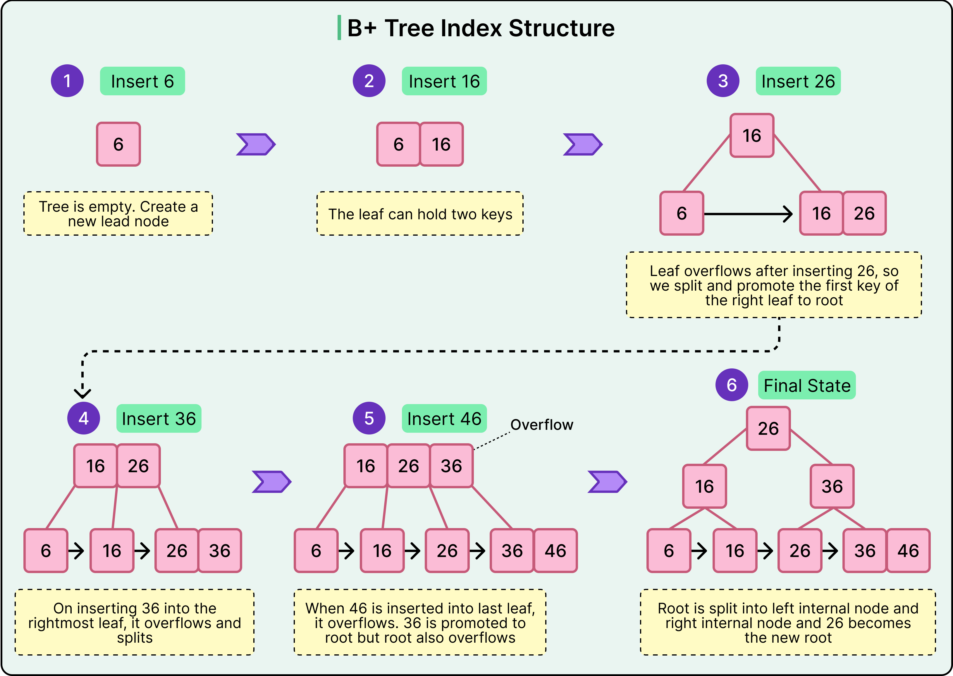
Deletions work similarly in reverse. If a node becomes too empty, it may borrow from a sibling or merge with it. This rebalancing ensures that the tree remains efficient even as the data changes.
Performance Patterns and Pitfalls
B+ Trees are excellent for both equality and range-based queries. They support fast lookups on indexed columns and enable efficient scans across sorted ranges. This makes them well-suited for use cases like filtering by primary key, scanning by date, or paginating ordered results.
However, they perform poorly when the indexed column has low selectivity. For example, indexing a boolean column like is_active offers little benefit because the index points to a large portion of the table. In such cases, the engine may choose a full table scan over using the index.
Insert performance is also sensitive to key distribution. Sequential keys like auto-incrementing IDs perform well because new entries go to the rightmost leaf.
Hash Indexes
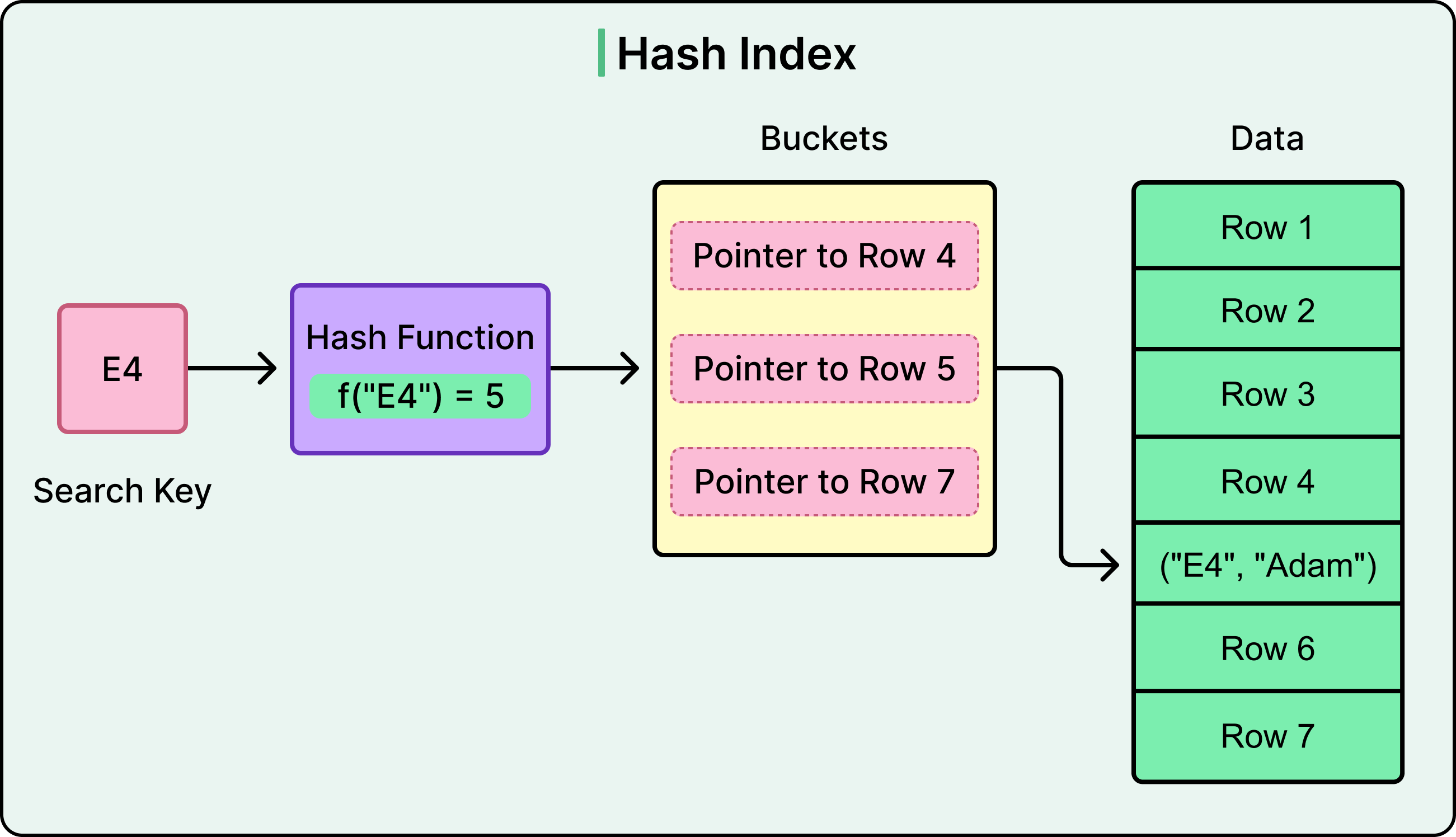
A hash index uses a hash function to map key values to fixed-size buckets. Each bucket stores a pointer, or a list of pointers, to the row(s) associated with that hashed key.
When a new key is inserted, the hash function computes a numeric value based on that key. This value determines which bucket the key-value pair is placed into. When a query searches for a specific value, the same hash function computes the bucket location again and retrieves tata directly from that slot.
See the diagram below:
Hash indexes handle collisions (when two keys map to the same bucket) using either chaining (a linked list of values per bucket) or open addressing (probing nearby buckets until a free or matching slot is found). The choice of strategy affects performance under high load or uneven key distribution.
The performance characteristics of a hash index are as follows:
Lookup performance is very fast for exact matches. The engine calculates the hash, checks the bucket, and retrieves the row.
Insert performance is also efficient, as new keys are simply hashed and placed in the appropriate bucket.
Delete operations remove entries based on the same hash lookup.
Search time remains stable as data grows, assuming the hash function distributes keys evenly.
However, the structure does not preserve any ordering of keys. In such cases, the engine must fall back to a full table scan or another index.
Hash indexes are best suited for the following cases:
In-memory tables in which latency is critical.
Temporary data structures with known access patterns.
High-cardinality exact-match queries, such as searching by session token or API key.
Hash-based partitioning or sharding, where the goal is to distribute data evenly across nodes or files.
Limitations of the Hash Index
Hash indexes are also prone to load imbalance if the hash function is weak or if the data is skewed. Also, they consume more memory than tree-based indexes for equivalent functionality, especially when the number of buckets grows to avoid collisions.
Poor hash function design can lead to clustering, where too many keys fall into the same bucket, degrading performance and reducing lookup consistency. Resizing or rehashing the structure during growth phases can also lead to spikes in write amplification.
Bitmap Indexes
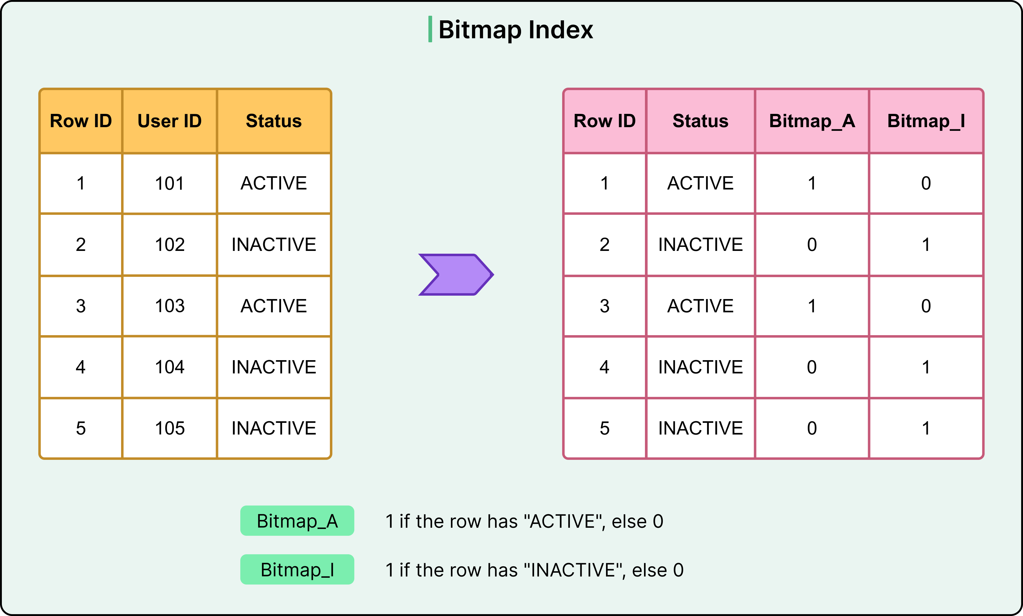
A bitmap index takes a different approach to indexing by representing data presence using bitmaps rather than tree or hash structures. For each distinct value in a column, the index maintains a bit vector: a sequence of bits where each bit corresponds to a row in the table. If the row has that value, the bit is set to 1; otherwise, it remains 0. This structure allows the database to evaluate complex filters quickly using bitwise logic, often with performance that tree-based indexes cannot match.
Imagine a gender column with two possible values: 'active' and 'inactive'. A bitmap index for this column would create two separate bitmaps: one for each value. If the table has 10,000 rows, each bitmap would be 10,000 bits long. A query filtering for 'active' can access the corresponding bitmap directly and identify all matching rows in a single scan.
The bitmaps align with row positions, allowing the engine to combine them efficiently using AND, OR, and NOT operations.
Consider the following query:
SELECT COUNT(*) FROM users
WHERE gender = 'F' AND status = 'active';
It can be resolved by performing a bitwise AND on the two relevant bitmaps, identifying matches without touching the base table.
Bitmap indexes are ideal for:
Columns with low cardinality, such as gender, status, or region.
Workloads where data is mostly static and read-focused.
Analytical platforms and data warehouses that benefit from multi-column filtering.
Limitations of Bitmap Indexes
Bitmap indexes shine in read-heavy, analytic environments where query performance depends on filtering across multiple columns. Because bitmaps are compact and bitwise operations are fast, queries can resolve complex conditions with minimal I/O. However, they struggle in transactional workloads. Updates, inserts, or deletes require modifying multiple bitmaps, which becomes costly at scale.
Write-heavy environments introduce overhead because every bitvector must be adjusted whenever a change is made. This slows down operations and can cause contention in concurrent workloads.
Bitmap indexes are not a fit for high-cardinality columns, such as user_id or email. The number of bitmaps would grow linearly with the number of distinct values, leading to excessive memory usage.
Inverted Indexes
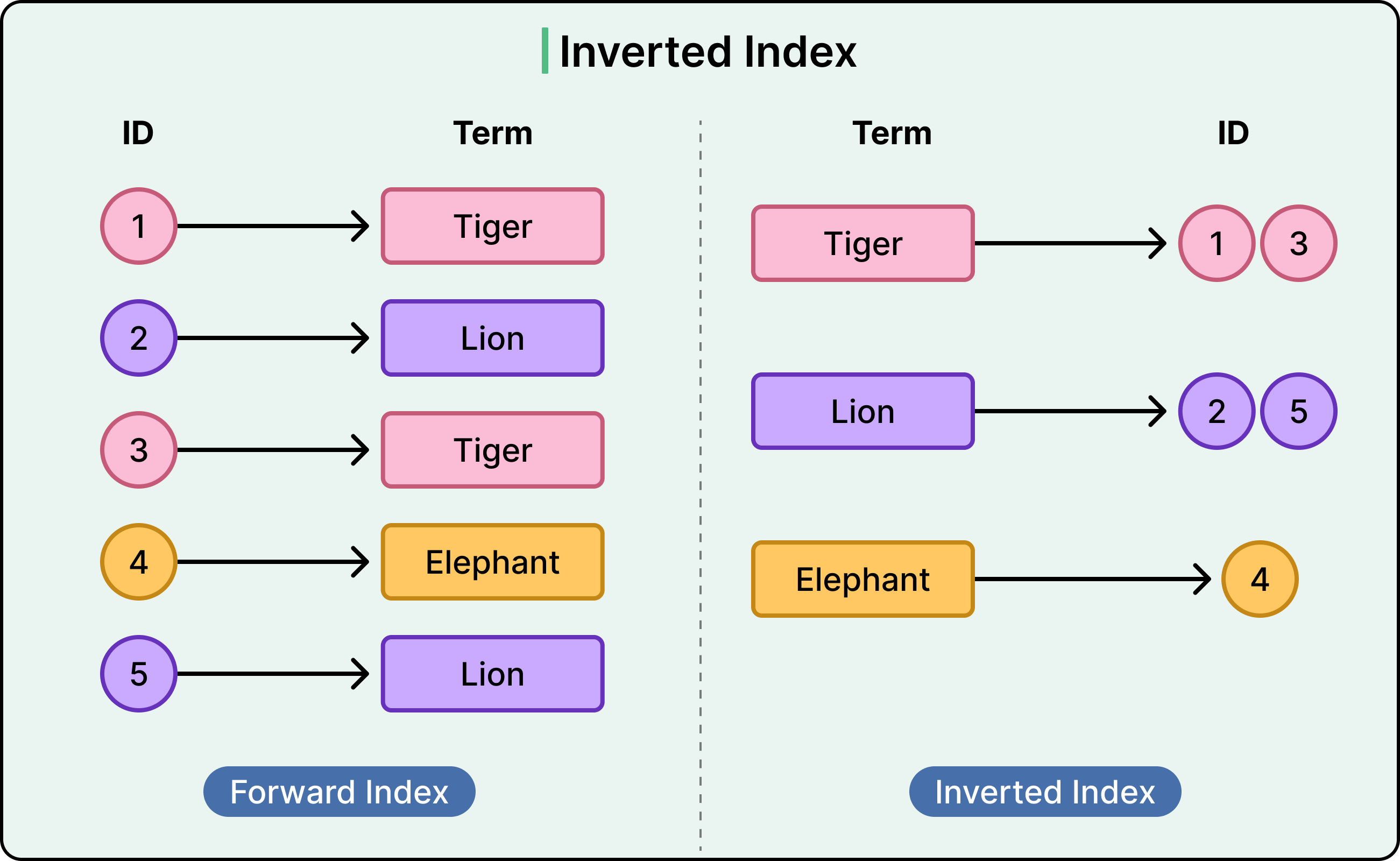
An inverted index flips the typical indexing model. Instead of mapping rows to values, it maps specific terms to the documents or rows where those terms appear. This design is optimized for full-text search and excels at querying large volumes of unstructured or semi-structured text.
See the diagram below
The process starts with tokenization. The database or search engine breaks input text into individual terms, or tokens, usually by splitting on whitespace and punctuation, then applying filters like case normalization.
For each token, it records a list of documents (or rows) that contain that term. As an example, the term “database” might map to:
"database" → [doc_1, doc_4, doc_19]Updates and deletions require modifying the lists. Adding a document involves tokenizing it and updating each relevant list. Removing a document means purging it from all lists where it appears. This process is efficient but not instantaneous, so many systems handle it in batches or via background processes.
Inverted indexes are built into many systems:
MySQL supports full-text indexes using its FULLTEXT keyword.
PostgreSQL offers full-text search using “tsvector” and “tsquery”, with support for dictionaries, stopwords, and ranking.
Elasticsearch is built entirely around inverted indexes and supports full-text search, filtering, and aggregations at scale.
Limitations of Inverted Indexes
Inverted indexes are highly specialized. They are not a replacement for traditional indexes and are not suitable for structured queries like equality lookups or range filters on numeric columns.
They also demand careful handling of:
Stemming, to group words like "run" and "running".
Stopwords, which remove common terms like "the" or "and".
Language support, especially in multilingual datasets.
Without proper configuration, these details can skew relevance scores or omit valid matches.
Summary
In this article, we’ve looked at database index internals and the data structures that power them in detail.
Here are the key learning points in brief:
Index structures define how databases locate data efficiently without scanning entire tables. Different structures are optimized for different access patterns.
A B+ Tree is the default indexing structure in most relational databases. It stores all values in leaf nodes and supports fast lookups, range queries, and ordered scans. It also maintains logarithmic search time through balanced branching and efficient node splitting and merging during inserts and deletes.
B+ Trees perform well on selective queries but degrade when used on unselective predicates. Inserts can suffer when random keys like UUIDs cause frequent page splits.
Hash indexes use a hash function to map keys to buckets and offer near-constant time performance for exact-match lookups.
Hash indexes are unsuitable for range queries or sorting, and they can suffer from poor distribution if the hash function is weak or the data is skewed.
Bitmap indexes use a bit vector per distinct column value, enabling fast filtering using bitwise operations on low-cardinality columns.
Bitmap indexes are ideal for analytic workloads in data warehouses but introduce high write overhead and are unsuitable for transactional systems or high-cardinality fields.
Inverted indexes map terms to documents and are used in full-text search systems. They tokenize input text and build posting lists for fast term-based retrieval.
These indexes are common in systems like Elasticsearch and full-text features in PostgreSQL and MySQL, but they are not appropriate for structured numeric or range queries.
Each index structure introduces trade-offs in read performance, write cost, memory usage, and query flexibility. Choosing the right one depends on access patterns and workload characteristics.


typo: "retrieves tata directly from that slot"
data?