Database schema design plays a crucial role in determining how quickly queries run, how easily features are implemented, and how well things perform at scale. Schema design is never static. What works at 10K users might collapse at 10 million. The best architects revisit schema choices, adapting structure to scale, shape, and current system goals.

Done right, schema design can become a great asset for the system. It accelerates product velocity, reduces data duplication debt, and shields teams from late-stage refactors. Done wrong, it bottlenecks everything: performance, evolution, and sometimes entire features.

Every engineering team hits the same fork in the road: normalize the schema for clean structure and consistency, or denormalize for speed and simplicity. The wrong choice doesn’t necessarily cause immediate issues. However, problems creep in through slow queries, fragile migrations, and data bugs that surface months later during a traffic spike or product pivot.

In truth, normalization and denormalization aren't rival approaches, but just tools to get the job done. Each solves a different kind of problem. Normalization focuses on data integrity, minimal redundancy, and long-term maintainability. Denormalization prioritizes read efficiency, simplicity of access, and performance under load.

In this article, we’ll look into both of them in detail. We’ll start with the foundations: normal forms and how they shape normalized schemas. We will then explore denormalization and the common strategies for implementing it. From there, we will map the trade-offs between normalization and denormalization

The goal isn't to declare one approach as the winner. It's to understand their mechanics, consequences, and ideal use cases. 

Foundations of Schema Design

Schema design sets the foundation for how a system stores, relates, and retrieves data. Let’s understand a few key aspects about it in detail.

What Is Schema Design?

Schema design is the structural blueprint of a relational database. 

It defines what tables exist, how they relate to each other, and what rules govern their data. 

A well-designed schema enforces integrity, reduces duplication, and enables efficient querying. The best schema designs reflect both the business domain and the access patterns of the application. 

The Role of Entity-Relationship Modeling

Before defining tables, schema design typically starts with Entity-Relationship (ER) modeling. 

This high-level design process maps out entities (real-world objects or concepts), their attributes (data fields), and the relationships between them.

ER models help clarify cardinality (one-to-many, many-to-many) and participation constraints (mandatory vs. optional relationships). These details drive the eventual table structure and foreign key decisions. Most importantly, ER modeling sets the stage for normalization by identifying the core units of meaning in the data model.

Logical vs. Physical Schema

The logical schema defines the data model at a conceptual level (tables, columns, keys, and relationships) without worrying about how the database engine will implement it. The physical schema, on the other hand, involves indexes, partitioning strategies, storage engines, and disk layout.

That separation matters. 

A schema might look clean on paper, but perform poorly in production. Performance tuning often begins with the logical schema, but ends in the physical layer. Understanding both is critical when navigating trade-offs between normalization and denormalization later in the stack. For this article, we’ll stay in the logical space. 

Normalization

Normalization sits at the heart of relational database design. It’s a methodical process that shapes how data is structured, stored, and maintained.

At its core, normalization aims to eliminate data redundancy. Storing the same information in multiple places might seem convenient at first, but it invites inconsistencies and increases storage needs. A normalized schema stores each piece of information exactly once, then references it wherever needed.

The second goal is to prevent update anomalies. Without normalization, modifying a single data point (like changing a product name or a user email) might require updating multiple rows in different tables. Miss one, and the data becomes inconsistent. Normalization ensures that updates propagate correctly and predictably.

Finally, normalization enforces logical data dependencies. It ensures that every column in a table relates directly to the primary key, not indirectly through some unrelated field. This clarity makes the data model easier to reason about, test, and evolve.

In short, normalization brings structure. When applied correctly, normalization makes schemas lean, predictable, and resilient to change. When ignored or misused, it can lead to bloated tables, hidden dependencies, and a maintenance nightmare.

The Normal Forms

Normal forms are a set of rules used to improve database design. Each form targets a specific kind of redundancy or anomaly.

Let’s look at different normal forms with examples.

1 - First Normal Form (1NF)

1NF requires that:

• Each column contains a single, atomic value.

• No column contains a set, list, or repeating group. In other words, each column in a table must contain only one value in a cell. For example, a value like “productA, productB” in one column violates the first normal form.

Consider a raw orders table as shown in the diagram below.

The problem here is clear. Multiple products live in separate columns. This design violates 1NF because it contains multiple columns (Product1, Product2, and Product3) that refer to the same type of data. To fix it, break out each product into a separate row as shown in the diagram below:

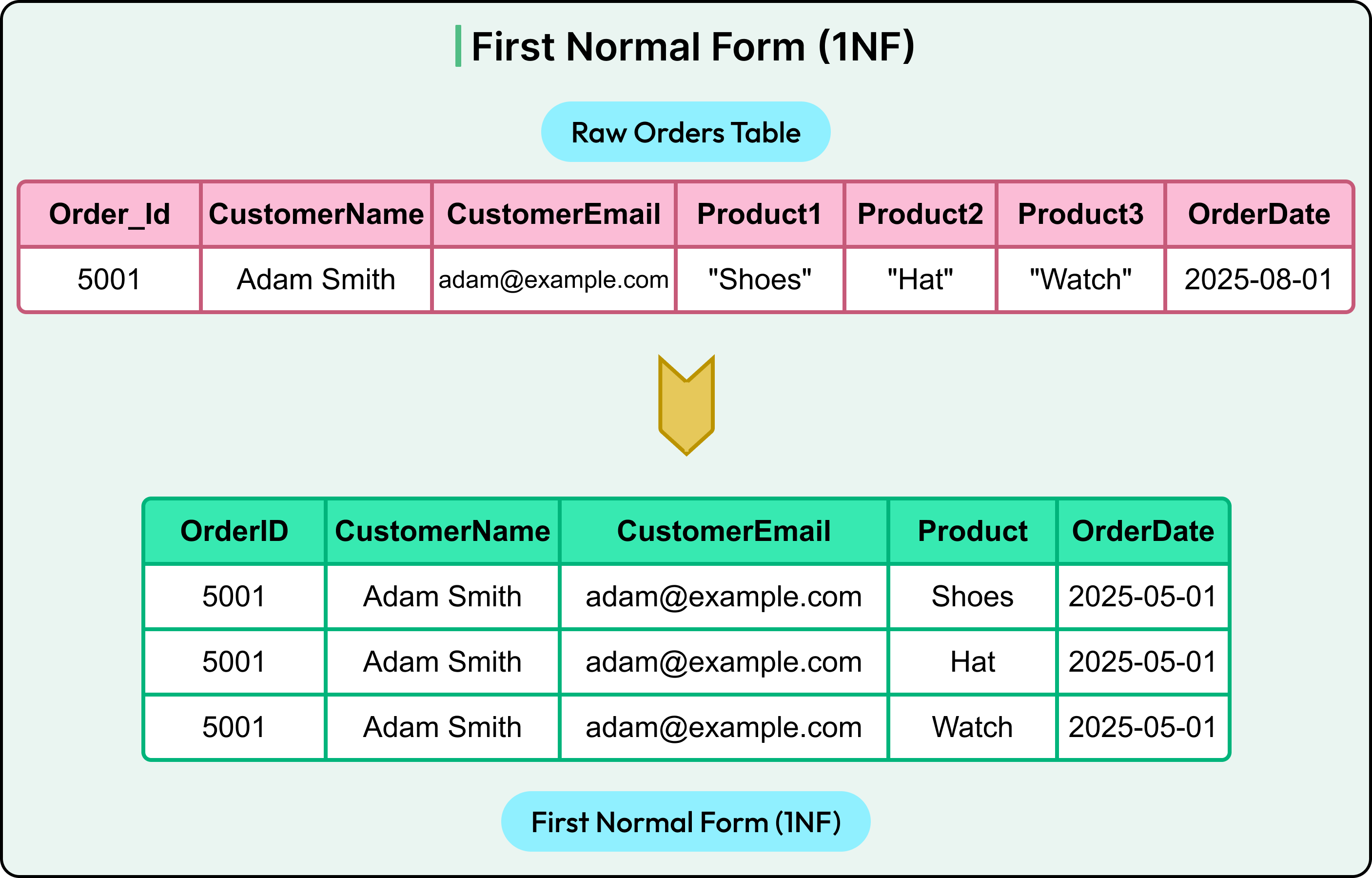
Now the table is in 1NF. Each column holds a single value, and the product data is no longer spread across multiple fields.

2 - Second Normal Form (2NF)

2NF builds on 1NF by requiring that all non-key columns depend on the entire primary key, not just part of it. In other words, it eliminates partial dependencies.

Assume the primary key here is a composite of (OrderID + Product) in the current structure. In that case, columns like CustomerName and CustomerEmail depend only on OrderID, not the full key. That’s a partial dependency.

To adhere to 2NF, split the data into two tables as shown in the diagram below:

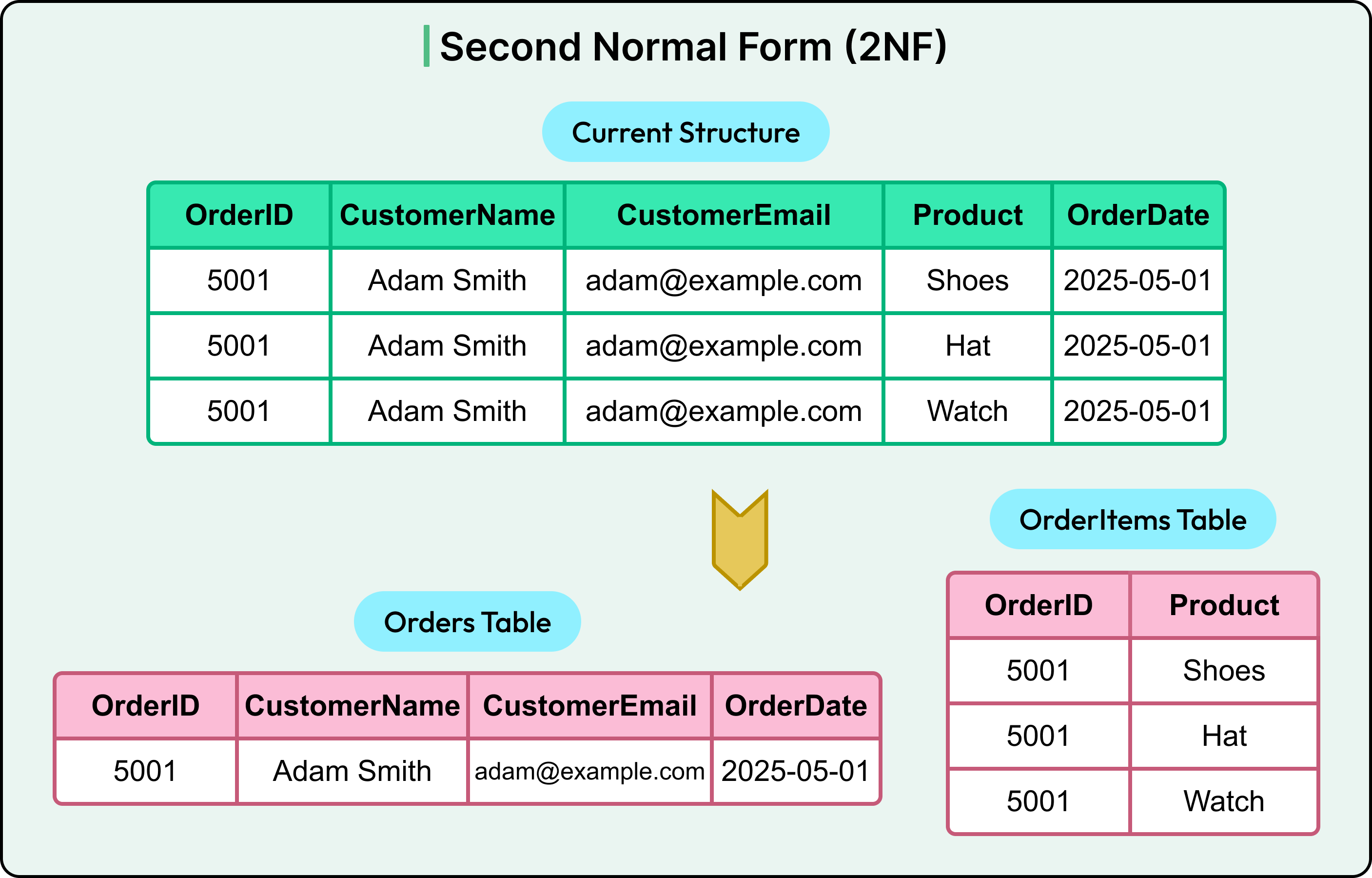
Now, every non-key column in each table depends fully on the primary key. The schema is in 2NF.

3 - Third Normal Form (3NF)

The third normal form is a key concept of database normalization. 3NF eliminates transitive dependencies when a non-key column depends on another non-key column.

Let’s say the system adds a Region column inferred from the email domain.  Here, Region is indirectly dependent on CustomerEmail and not directly on OrderID. That’s a transitive dependency.

To bring this into 3NF, break the customer information into a separate table as shown in the diagram below:

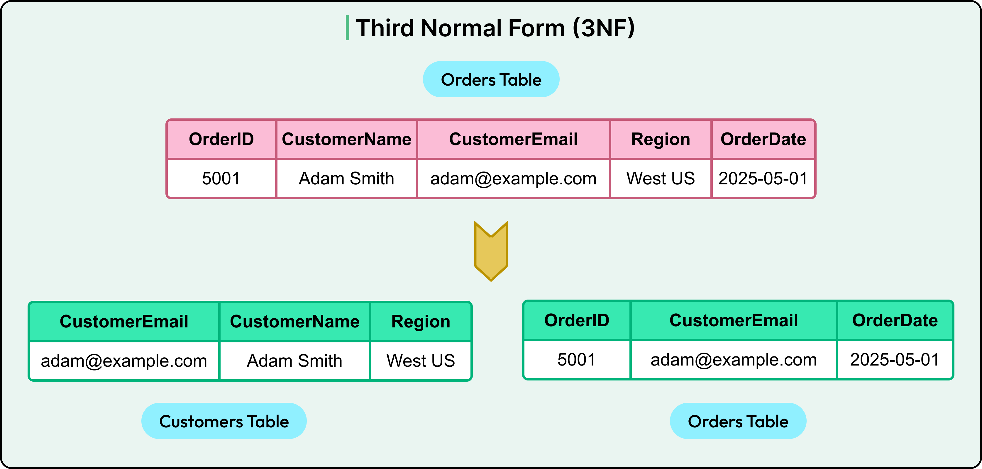
Now, each non-key column depends only on the primary key in the respective table. The schema satisfies 3NF.

4 - Boyce-Codd Normal Form (BCNF)

BCNF addresses a rare edge case where 3NF passes, but anomalies still exist due to overlapping candidate keys.

Imagine a table where each row represents a course being taught in a specific room. It looks something like this:

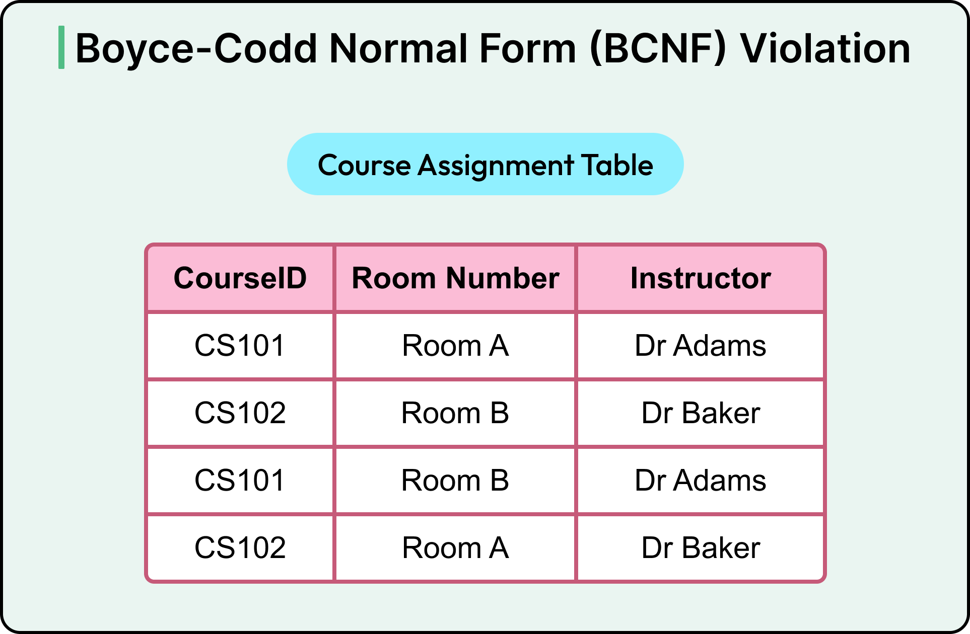
Now, based on how this system works, there are two facts to know:

• Each course is always taught by the same instructor, no matter which room it’s scheduled in. For example, CS101 is always taught by Dr Adams, whether it happens in Room A or Room B.

• Each room can only be used for one course at a time. So if Room A is booked at a certain time, it can only be used for one course in that slot (for example, CS101).

In other words, there are two key relationships here:

• If the Course ID is known, the Instructor can be looked up. In other words, the identity of the course fully determines which instructor is teaching it.

• If the Room Number is known (during a specific time), the Course ID being taught there can be determined. That is, the room tells us which course is being taught in it.

At first glance, this might seem fine. But imagine what happens if someone updates the instructor for CS101 in only one of the rows and forgets the other. Suddenly, CS101 appears to be taught by two different people.

This is because the Instructor depends only on the Course ID, not on the combination of the Course ID and the Room Number. Therefore, storing the instructor repeatedly across multiple rows opens the door for inconsistencies. The moment the same course shows up in different rooms, there’s a risk that someone might assign different instructors by mistake.

This violates BCNF. 

In relational design terms, the primary key of this table is a combination of Course ID and Room Number because each row is meant to describe a specific pairing of a course in a room. However, the problem is that one of the columns, Instructor, doesn’t depend on both of those values. It depends only on the Course ID. 

That’s a mismatch.

BCNF says that if a column depends on some other column, then that “other column” must be enough to identify each row on its own uniquely. In other words, it must be a key. 

In this case, Course ID determines the Instructor, but Course ID is not the table’s key. The key is the Course ID and Room Number. Therefore, we’ve a dependency that doesn’t align with the key.

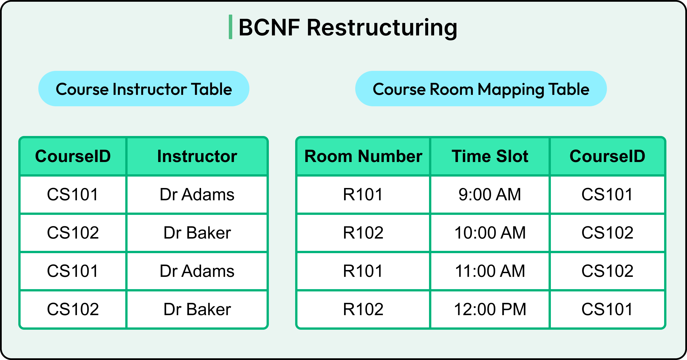
The fix is to split the table into two separate ones that reflect the actual relationships in the data. See the diagram below, where we have two tables: Course Instructor and Course Room Mapping. The Course Room Mapping table has R101 (Room A) and R102 (Room B) to map the Course ID with the time slot.

5 - Fourth Normal Form (4NF)

4NF comes into play when a single table tries to represent two or more independent one-to-many relationships for the same entity. It ends up generating all possible combinations, resulting in a Cartesian explosion.

For example, let’s say there is an employee E001 who knows two skills: Java and Python. Also, E001 is working on two projects: ProjectX and ProjectY. 

How many rows are needed to represent all this in one table with three columns: EmployeeID, Skill, and Project?

The answer is 4 rows because the table doesn’t know whether a skill applies to a specific project or not. Therefore, it assumes every skill is used in every project, resulting in the Cartesian explosion. The situation only gets worse with more skills and projects.

This structure seems to suggest that an employee is using Java on ProjectY and Python on ProjectX. However, it may not be true, and the company never recorded which skill is used on which project, and doesn’t even care. However, the table is implying relationships that may not exist, which may be incorrect and also a waste of storage.

The skills of an employee and the project an employee is working on are two independent dimensions. And hence, it’s better to model them in independent tables. 

See the diagram below:

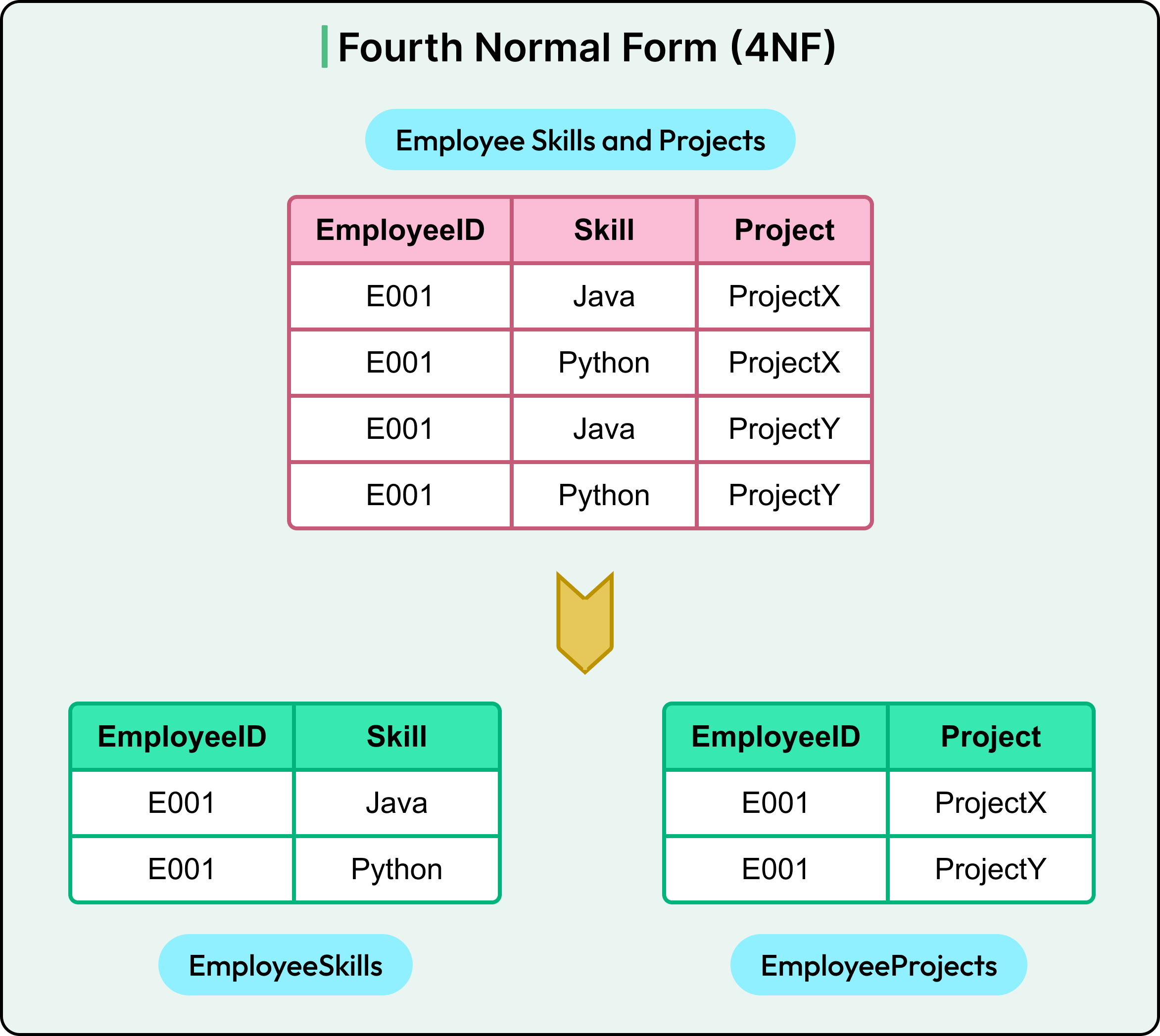
This is the 4NF approach that eliminates redundant combinations from multi-valued dependencies.

Takeaway

The first three forms (1NF, 2NF, and 3NF) handle 95% of real-world use cases. 

They ensure data is stored logically, with minimal redundancy and maximum integrity. BCNF adds guardrails for edge cases, while 4NF and other higher normal forms deal with complex many-to-many and join-heavy designs.

Denormalization

Denormalization flips the principles of normalization on their head.

While normalization brings structure and integrity, it often comes at a performance cost. Denormalization introduces controlled redundancy to reduce that cost, especially in read-heavy systems where query speed matters more than strict normalization rules.

Normalized schemas often require multiple joins to fetch a complete data object. This works fine at a low scale. But as traffic grows, or query complexity deepens, those joins can become bottlenecks.

Consider a product dashboard that pulls:

• User details from a Users table.

• Product data from Products.

• Order info from Orders.

• Discount info from a Promotions table.

A normalized schema requires four joins to assemble the view. At scale, these joins hit disk, strain indexes, and increase query latency.

Denormalization addresses this by pre-joining or duplicating data. It puts everything the application needs into a single place, so the database has to do less work during reads. In other words, denormalization trades write complexity for read performance.

Common Denormalization Techniques

Denormalization isn’t one-size-fits-all. 

It takes different forms depending on access patterns, performance goals, and database constraints. 

Below are common patterns used in production systems:

1 - Merging Related Tables

The simplest approach is to combine two frequently joined tables into one. For example, if every order needs customer data, consider merging Orders and Customers.

See the diagram below for reference:

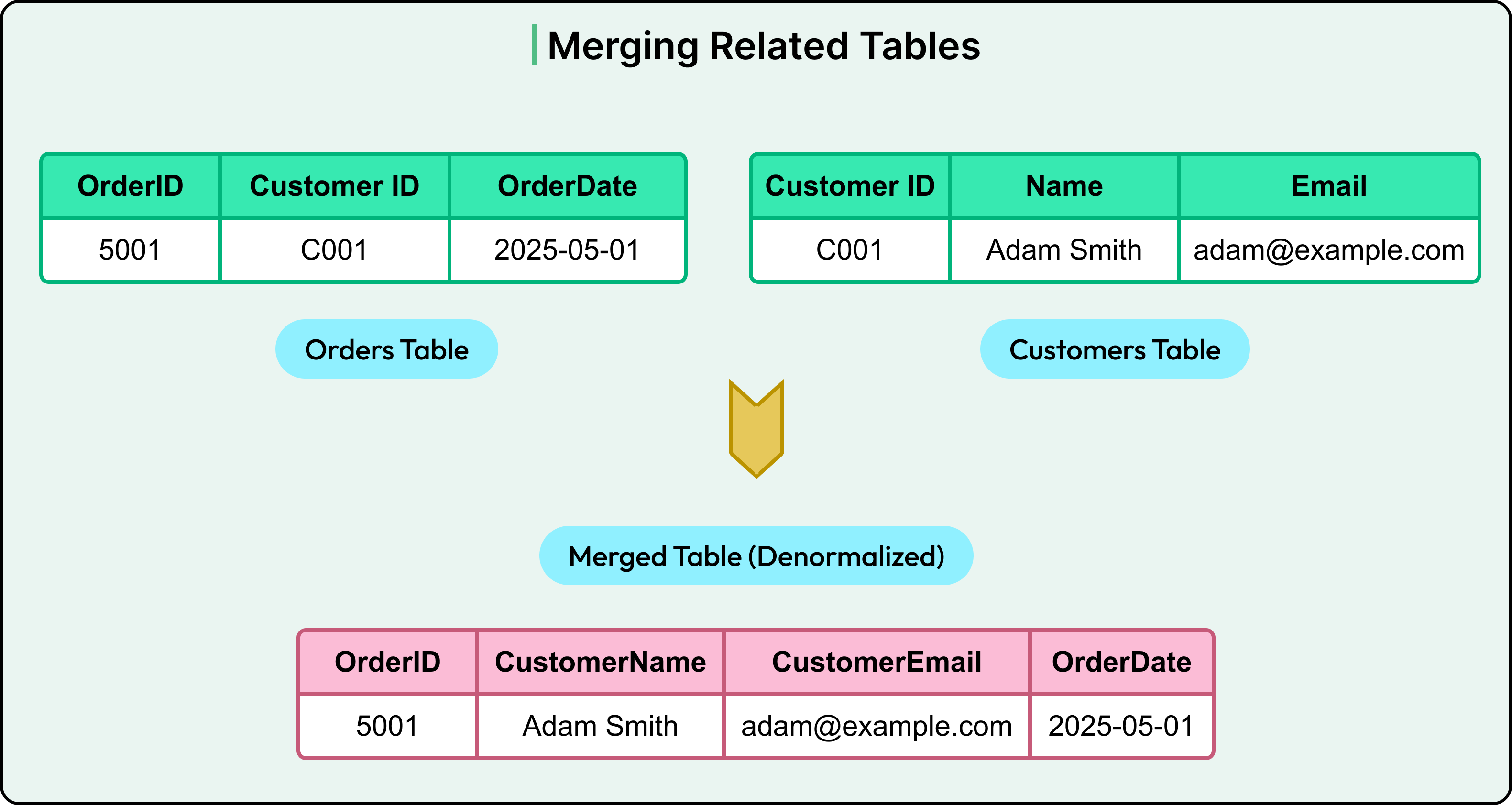
Now, reading an order no longer requires a join. But updating a customer’s name means touching every order they've placed.

The trade-off is that this approach is great for read speed. However, it can be problematic if customer details change frequently.

2 - Add Redundant Columns

Sometimes, full merging isn’t needed, and just selective duplication is sufficient. 

For example, storing ProductName in the OrderItems table, even though Products already holds that information.

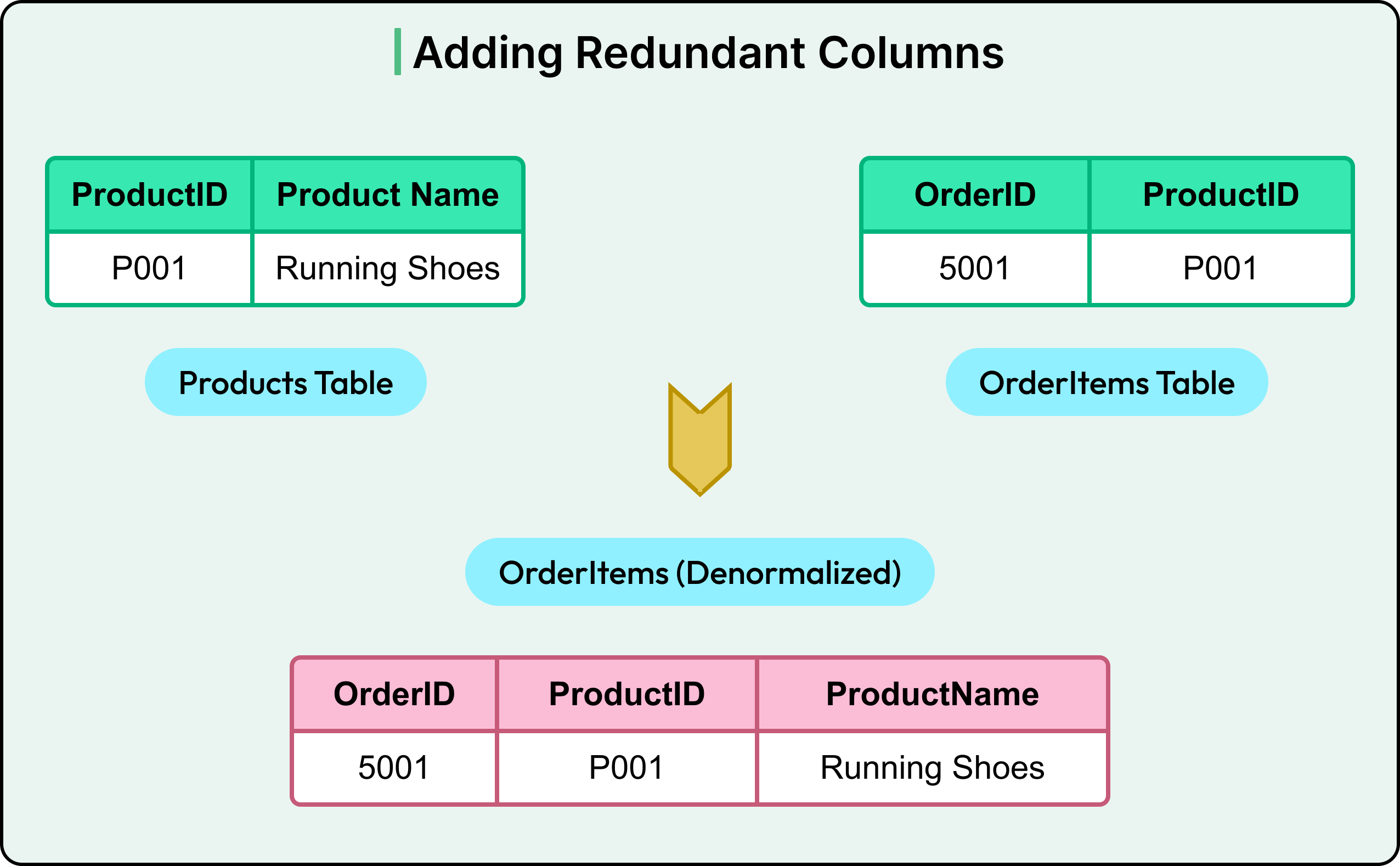
This avoids a join at query time, especially useful in reporting or data export scenarios. However, if product names change (for example, due to branding), every reference needs an update.

The trade-off here is faster reads, but at the risk of stale or inconsistent data.

3 - Creating Summary Tables

Summary tables pre-aggregate data to avoid expensive computations during reads.

This structure is ideal for dashboards and analytics tools. Updates are handled via scheduled jobs, event triggers, or batch pipelines.

The trade-off here is fast queries at the cost of freshness. However, it needs orchestration to stay accurate.

4 - Using Materialized Views

Materialized views store the output of a query, not just the query itself. They’re maintained by the database and can be refreshed periodically or incrementally.

CREATE MATERIALIZED VIEW TopProducts AS
SELECT ProductID, COUNT(*) AS OrderCount
FROM OrderItems
GROUP BY ProductID;

Now, getting top-selling products becomes a simple “select” query. Most relational databases (for example, PostgreSQL, Oracle) support this.

See the diagram below that shows the basic concept of a materialized view with another example where a specific value can be calculated and stored for quick and efficient queries:

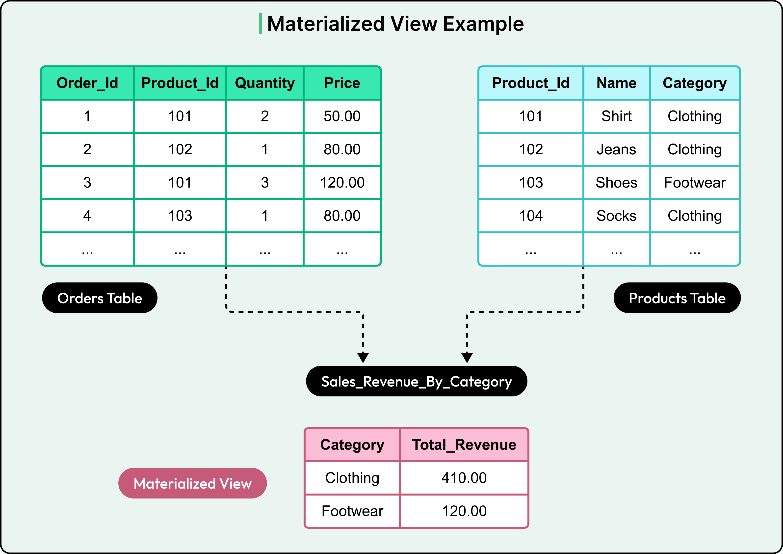
The trade-off is that materialized views simplify queries and offload computation, but they need careful refresh logic. Stale views can mislead consumers.

Trade-Offs Between Normalization and Denormalization

Let’s look at some of the key trade-offs involved when choosing between normalization and denormalization.

Performance Considerations

Normalized schemas shine when it comes to write performance and data integrity. Since data lives in one place, insertions and updates are efficient and safe. There's no need to write the same value into multiple tables or worry about consistency across redundant fields.

However, reading normalized data often involves multiple joins, especially in feature-rich applications. That means:

• More CPU cycles per query,

• More disk seeks for scattered rows,

• And more room for subtle performance regressions as the data grows.

Denormalized schemas flip the equation. By duplicating data or storing pre-joined structures, they eliminate joins at query time, dramatically reducing response times. This is especially useful for dashboards, search APIs, and mobile clients where latency is king.

Maintenance Complexity

Normalized data models are easier to evolve and maintain. Changing a data attribute (like renaming a product or updating a user’s profile) happens in one place. Indexes and constraints stay lean. Also, refactoring a schema doesn’t involve hunting down duplicated logic or scattered dependencies.

Denormalized schemas are harder to keep consistent. Data duplication means more places to update. Every new sync path introduces the risk of bugs, missed edge cases, or stale values leaking into production.

In practice, keeping denormalized data clean requires:

• Custom update logic.

• Scheduled jobs or triggers.

• Change-data-capture pipelines.

All of these add engineering overhead and failure points.

Storage and Redundancy

Normalized schemas are space-efficient. Each data item is stored once, indexed as needed, and referenced by keys. In large-scale systems with high write volumes, like messaging apps or transaction logs, this efficiency compounds quickly.

Denormalized schemas utilize more space by design. Redundant fields, summary tables, and precomputed joins all inflate disk usage. However, in read-optimized environments like OLAP systems or data warehouses, that trade-off is often acceptable.

Use-Case-Driven Decision Making

There’s no universal “correct” level of normalization. It depends entirely on how the system behaves.

• OLTP systems (such as banking, e-commerce, and inventory management) deal with frequent writes, strict consistency, and transactional integrity. Here, normalization works best.

• OLAP systems (such as reporting dashboards, customer insights, and event analytics) prioritize fast reads and aggregations across large datasets. Denormalization, summaries, and precomputed joins help them scale.

In many cases, the answer lies somewhere in between. Teams normalize the core schema, then selectively denormalize read-critical paths either manually or through caching layers, materialized views, or downstream data platforms.

Best Practices For Developers

Schema design isn’t a one-and-done task, but a continuous process. Workloads shift, access patterns evolve, and what worked at launch might struggle under growth. 

Some best practices that can help developers are as follows:

Start with Normalization, Denormalize Later

Start with a clean, normalized schema. It clarifies intent, enforces consistency, and makes the data model easier to reason about. Early-stage systems benefit from this clarity, especially when the domain is still evolving or when correctness matters more than speed.

Denormalize only in response to specific requirements. If a specific read path becomes a bottleneck and joins become costly, denormalize that slice of the model.

Monitor Query Patterns and Workload Behavior

Schema design without observability is equivalent to guesswork. Use query logs, slow query analyzers, APM tools, and database profilers to spot the real hotspots.

Look for patterns like:

• Frequent joins across the same set of tables

• High latency on aggregate queries

• Heavy reads on fields that require lookups or subqueries

Use these signals to validate whether denormalization will improve performance. 

Automate Consistency Where Possible

Denormalization always introduces the risk of stale or inconsistent data. When choosing to duplicate data across tables or systems, automate consistency as much as possible.

Some options include:

• Triggers: Use database-level triggers to propagate changes. This is effective for low-frequency updates but hard to maintain at scale.

• Application logic: Centralized writes in well-defined service layers that update all relevant tables in sync.

• Background jobs: Periodically refresh derived or summary data to correct drift in eventual consistency models.

• Change Data Capture (CDC): Stream changes from the source of truth to downstream copies in real-time or near-real-time pipelines.

Summary

We’ve now looked at database schema design with special focus on normalization and denormalization in detail.

Here are the key learning points in brief:

• Schema design defines how data is structured, related, and retrieved in a database, impacting performance, maintainability, and correctness.

• Entity-Relationship (ER) modeling helps identify entities, attributes, and relationships, forming the conceptual basis for table design.

• Logical schema focuses on data relationships and structure, whereas physical schema deals with how data is stored and optimized for performance.

• Normalization eliminates redundancy and enforces data integrity by organizing data into logical, dependency-driven forms.

• First Normal Form (1NF) removes repeating groups and ensures atomic values in each column.

• Second Normal Form (2NF) removes partial dependencies by ensuring all non-key columns depend on the full primary key.

• Third Normal Form (3NF) eliminates transitive dependencies, ensuring non-key columns depend only on primary keys.

• Boyce-Codd Normal Form (BCNF) resolves edge cases involving multiple overlapping candidate keys.

• Denormalization introduces controlled redundancy to optimize for read-heavy workloads by reducing joins and simplifying queries.

• Common denormalization techniques include merging tables, duplicating fields, creating summary tables, and using materialized views.

• Normalized schemas improve write performance and data consistency but often suffer from slower reads due to costly joins.

• Denormalized schemas optimize for read speed but introduce complexity in writes and data consistency management.

• Normalized models are easier to maintain, while denormalized ones require tooling or specific logic to keep redundant data accurate.

• Storage use is leaner in normalized schemas, whereas denormalization trades disk space for performance and developer convenience.

• OLTP systems favor normalization for consistency. On the other hand, OLAP systems lean on denormalization to serve complex, high-volume reads efficiently.